WEB PAPER · 2026 MCM/ICM · PROBLEM F
Impact of AI on Employment: A Blessing or a Curse?
Team 2306116 · Honorable Mention
论文正文与参考文献的网页阅读版,保留提交稿的原图、表格和公式。
宽表格与长公式可横向查看;点击图片查看原图。
Summary
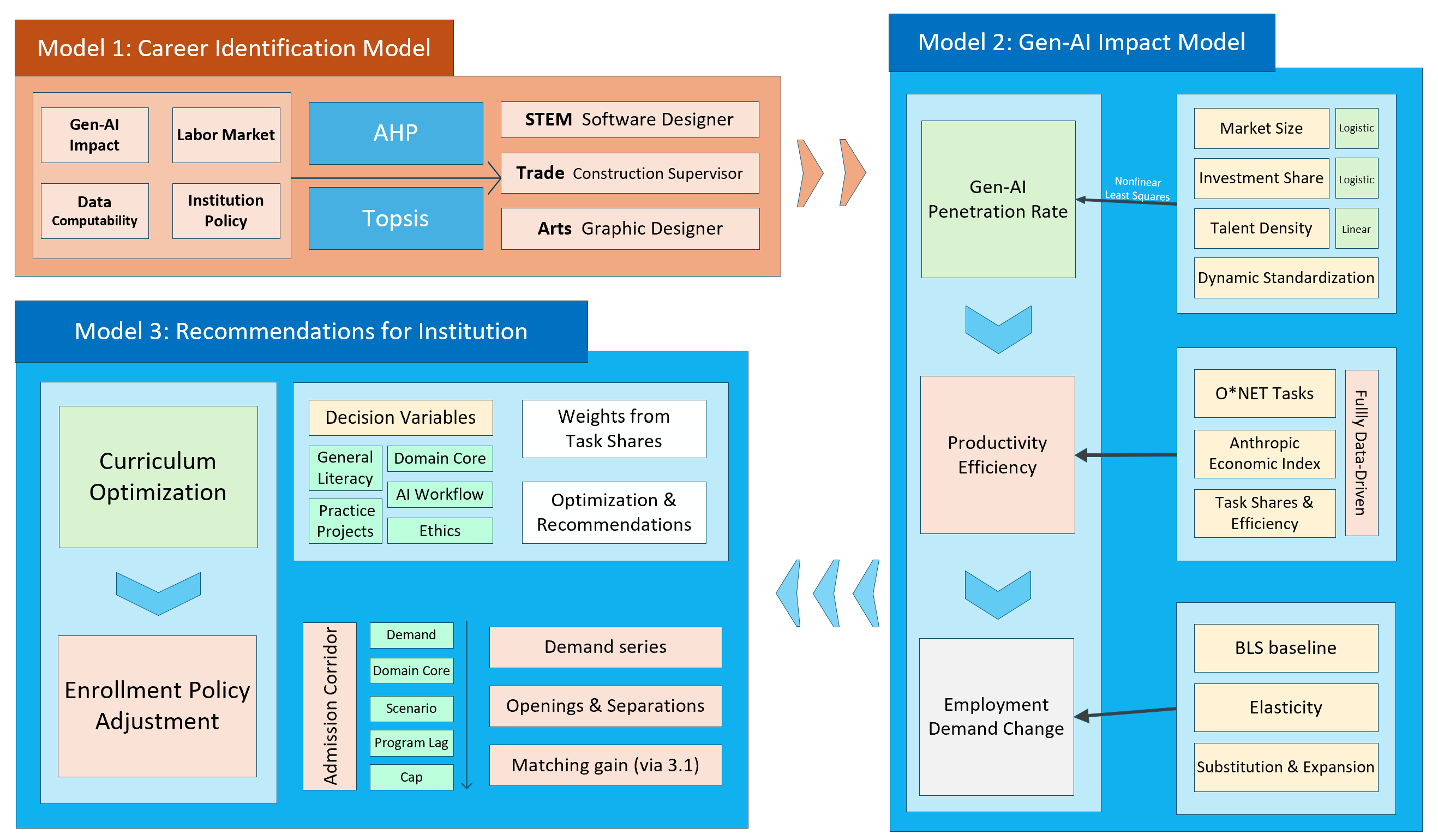
Generative artificial intelligence (Gen-AI) has exerted profound influence on future employment landscapes. Therefore, higher education institutions must adapt curricula to prepare graduates for significant challenges posed by Gen-AI. How should specific post-secondary institutions enhance graduate employability while effectively navigating Gen-AI? We have developed three models analyzing the future trajectories of each career category under Gen-AI's influence, and provide bespoke advice for selected institutions to navigate the implications of Gen-AI.
For question 1, we need to select one occupation from each of the categories: STEM, Trade, and Arts. We created the Career Identification Model (CI Model) using Analytic Hierarchy Process (AHP) and TOPSIS. Within the model, we evaluated and scored 18 occupations. Among these, Software Engineer, Construction Supervisor, and Graphic Designer ranked first within their respective fields of STEM, Trade, and Arts, achieving scores of approximately 0.818, 0.912, and 0.682, respectively. In conclusion, we selected these three professions for further analysis.
For question 2, we must examine the future trajectory of our three selected professions under the current development path and anticipated impact of Gen-AI. To this end, we have established the Gen-AI Impact Model. Utilizing Logistic Regression and Linear Regression respectively, we analyzed the AI penetration rate across the three professions, thereby determining the impact of Gen-AI on productivity with the Dynamic Standardization Method. Enhanced productivity brings about shifts in employment demand. Through our Employment Demand Model, we arrive at the following conclusions: software engineers will experience employment expansion, construction supervisors may face contraction, while graphic designers are entering a period of fluctuating adjustment.
For question 3, we shall identify a specific higher education institution and its study program for each of the three occupations selected, and present recommendations to the institution's leadership on addressing Gen-AI within the study program. We optimized the curriculum by restructuring it into five modules: AI Foundations, Advanced Workflows, Ethical Governance, Domain Core, and Practical Internships. Findings suggest that software engineers should substantially increase advanced AI workflow training, construction supervisors should prioritize integrating on-site practice with AI tools, and graphic designers should focus on acquiring art-related design skills. Regarding admissions policy, we linked the Employment Demand model's employment projections to enrollment quotas. Considering the impact of curriculum reform, we established an Enrollment Planning model. Findings recommended moderate expansion for software engineers, steady growth for construction supervisors, and a cautious approach (quality over quantity) for graphic designers.
Keywords: Generative artificial intelligence (Gen-AI), Career Identification Model (CI Model), Analytic Hierarchy Process (AHP), TOPSIS, Gen-AI Impact Model, Logistic Regression, Linear Regression, Dynamic Standardization Method, Employment Demand Model, Curriculum Optimization, Enrollment Planning model
1 Introduction
1.1 Problem Background
With the rapid proliferation of Generative Artificial Intelligence (Gen-AI), its transformative impact has extended from niche technical domains to mainstream professional landscapes, reshaping the core demands of careers. However, a single educational strategy can not simultaneously address the triple imperatives of graduate employability, skill adaptability, and value alignment. We want to quantify Gen-AI’s effects on selected careers from each category, and give advice on Gen-AI-related knowledge and skills that educational institutions embed in their specialized programs to enhance graduate competitiveness.
To address these questions, we develop three integrated data-informed models. These analyses will balance Gen-AI’s utility and risks, align curriculum reforms with career trajectory shifts, and ensure recommendations account for both employability and holistic educational value.
1.2 Restatement of the Problem
Specifically, our study addresses the following three core problems:
Task 1: Choose particular careers: Select three careers respectively from the three given categories that are susceptible to the influence of Gen-AI.
Task 2: Design a data-informed model: Design a mathematical model to explore the future trajectory of each of the three selected careers, encompassing career development paths and the anticipated impact of Gen-AI.
Task 3: Propose advice for addressing Gen-AI: Provide three recommendations respectively for addressing Gen-AI, for the leaders of the institutions employing the three careers.
1.3 Our Work
For task 1, we first selected ten occupations from each of the three major occupational categories in accordance with the requirements of the task. Subsequently, we eliminated certain occupations using four feasibility indicators. Finally, we employed the AHP and the TOPSIS to screen out the three optimal careers.
For task 2, we first established analytical models for three observable metrics, subsequently employing these metrics to estimate the penetration rate of Gen-AI with the Dynamic Standardization Method. Next, we investigated the impact of Gen-AI on productivity. Finally, based on the projection that productivity gains will alter employment demand, we forecast the employment implications of Gen-AI for three occupations.
For task 3, we first undertook course optimization, restructuring the program into five modules: AI Foundations, Advanced Workflows, Ethical Governance, Domain Core, and Practical Internships. This analysis identified the key courses that individuals pursuing each of the three career paths should prioritize. Secondly, we established an admissions planning model to forecast enrollment numbers for training personnel across these three career streams, enabling higher education institutions to respond to future fluctuations in talent demand.
2 Model Preparations
2.1 Assumptions and Justification
This section lists general assumptions used for the career evaluation stage (Model 1: AHP + TOPSIS). They are stated here to keep the evaluation procedure well-defined and reproducible.
Fixed evaluation scope. All occupations are evaluated within the same scope (U.S. labor market context) and within a consistent reference window (recent/current data when available), ensuring cross-occupation comparability.
Indicator scale consistency. Each indicator score is mapped onto an integer scale from 1 to 5, where larger values mean “better” under that criterion. The mapping rules are applied uniformly across all occupations.
Comparability across occupations. Scores across different occupations are assumed comparable on the same 1–5 scale for each indicator (i.e., a “4” on A1 for occupation is comparable to a “4” on A1 for occupation ).
Independence for aggregation. Indicators may be correlated in reality, but for multi-criteria aggregation, we treat each indicator as a separate evaluation dimension and combine them using a common weight vector.
Stable preference weights. The relative importance of indicator groups and indicators (derived via AHP) is assumed to be stable during the evaluation stage and is applied consistently to all occupations.
Data sufficiency for scoring. Publicly available information is assumed sufficient to assign defensible scores for the selected indicators. For any ambiguous case, a conservative scoring rule is applied (do not overestimate).
2.2 Notations
The following symbols are only used for the career identification stage.
| Symbol | Type | Meaning |
|---|---|---|
| i | index | Occupation index, |
| j | index | Indicator index, . |
| k | index | AHP hierarchy index (group-level or within-group item index). |
| s i j | value | Raw score of occupation on indicator (1–5 scale). |
| 𝐒 | matrix | Score matrix of size . |
| w j | value | Global weight of indicator (AHP-derived, ). |
| 𝐰 | vector | Weight vector . |
| 𝐀 | matrix | AHP pairwise-comparison matrix (positive reciprocal). |
| 𝐰 ( A H P ) | vector | Priority vector extracted from (normalized). |
| C R | value | AHP consistency ratio for the pairwise-comparison matrix. |
| r i j | value | Normalized value used in TOPSIS for occupation on indicator . |
| v i j | value | Weighted normalized value in TOPSIS for occupation on indicator . |
| v j + , v j − | value | Positive / negative ideal solution components for indicator . |
| S i + , S i − | value | Distance of occupation to positive / negative ideal solutions. |
| C i | value | TOPSIS closeness coefficient for occupation (larger is better). |
3 Career Identification Model
3.1 Candidate Career
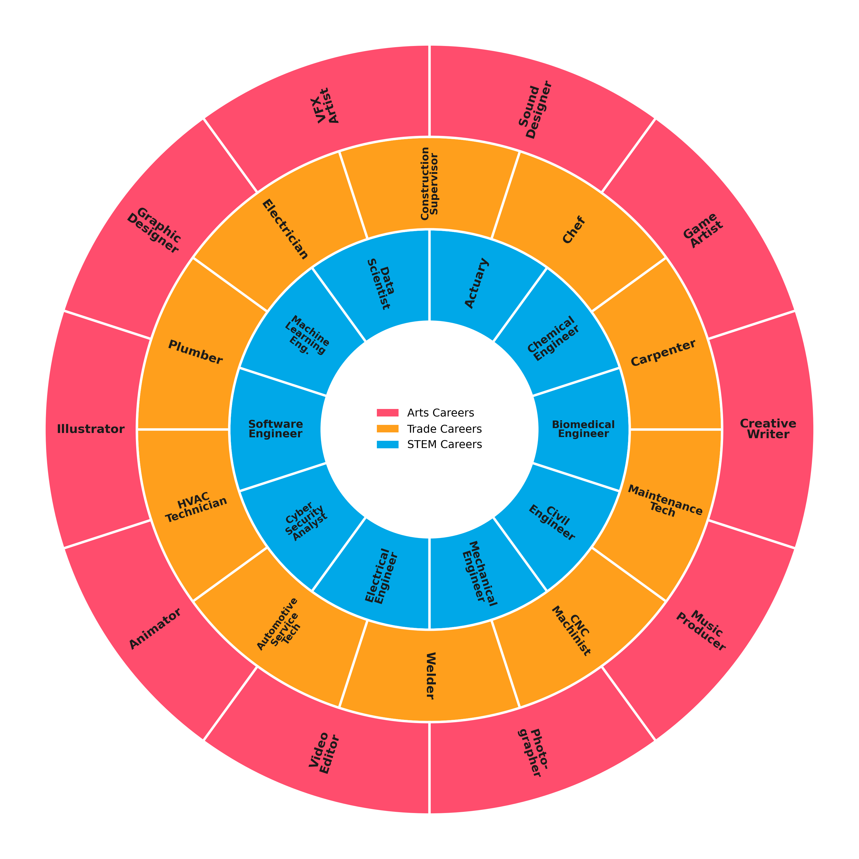
Firstly, we select ten careers from each of the following three categories: STEM career, Trade career and Arts career as shown in Figure 1. Then, we apply four hard constraints to conduct a preliminary screening of the selected careers. These constraints are as follows:
Project-specific binding: Must be clearly mappable to a specific institution and specific project
Data availability: Stable access to labor market and skill data
Clear Gen-AI mechanisms: At least 3 identifiable pathways for Gen-AI altering tasks/outputs/demands.
Educational leverage exists: Direct alignment of capability shifts through curricula, internships
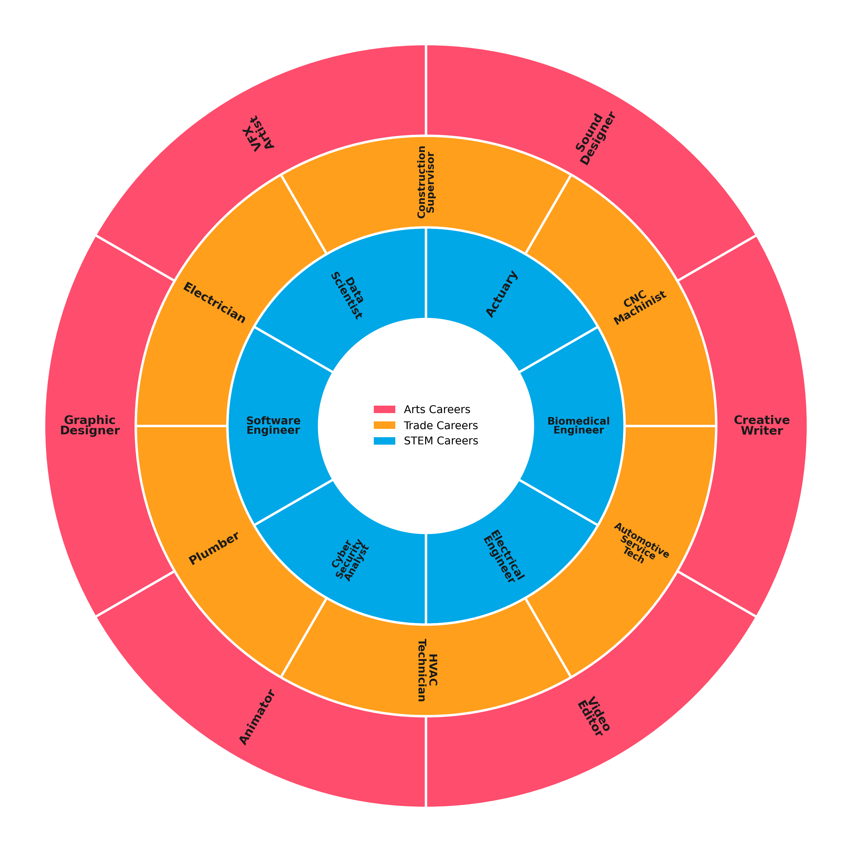
After filtering, we obtained 18 careers as shown in Figure 2:
3.2 Indicator System
Before we assess the aforementioned professions, we have established ten indicators, categorized into four groups. Each indicator is evaluated on a scale of 1 to 5, with a higher score indicating a greater degree to which the occupation fulfills that criterion.
| Group A | Group B | Group C | Group D |
|---|---|---|---|
| Gen-AI Impact | Labor Market | Data & Modeling | Institutional |
| A1: Automation Exposure A2: Augmentation A3: Adoption Speed | B1: Demand Scale B2: Wage & ROI | C1: Decomposability C2: Data Availability C3: Verifiability | D1: Controllable Course D2: Governance |
Based on the aforementioned ten indicators, we invite experts to help us score 18 careers:
| Profession | A1 | A2 | A3 | B1 | B2 | C1 | C2 | C3 | D1 | D2 |
|---|---|---|---|---|---|---|---|---|---|---|
| Data Scientist | 4 | 5 | 5 | 4 | 5 | 4 | 4 | 5 | 5 | 4 |
| Software Engineer | 5 | 5 | 5 | 4 | 5 | 5 | 5 | 5 | 5 | 4 |
| Cybersecurity Analyst | 4 | 4 | 4 | 4 | 5 | 4 | 5 | 4 | 5 | 5 |
| Electrical Engineer | 3 | 4 | 3 | 3 | 5 | 4 | 5 | 4 | 4 | 4 |
| Biomedical Engineer | 3 | 4 | 3 | 2 | 4 | 4 | 5 | 4 | 4 | 4 |
| Actuary | 4 | 4 | 4 | 4 | 5 | 5 | 5 | 5 | 4 | 5 |
| Electrician | 1 | 2 | 2 | 4 | 3 | 5 | 4 | 4 | 5 | 3 |
| Plumber | 1 | 2 | 2 | 3 | 3 | 5 | 4 | 4 | 5 | 2 |
| HVAC Technician | 1 | 2 | 2 | 4 | 2 | 5 | 4 | 4 | 5 | 3 |
| Automotive Service Technician | 1 | 2 | 2 | 4 | 2 | 5 | 4 | 4 | 5 | 2 |
| CNC Machinist | 2 | 3 | 3 | 3 | 2 | 5 | 4 | 4 | 5 | 2 |
| Construction Supervisor | 3 | 4 | 3 | 4 | 3 | 4 | 4 | 4 | 4 | 4 |
| Graphic Designer | 4 | 5 | 5 | 3 | 3 | 4 | 4 | 3 | 4 | 5 |
| Animator | 4 | 4 | 4 | 2 | 4 | 4 | 3 | 3 | 4 | 5 |
| Video Editor | 3 | 4 | 4 | 2 | 3 | 4 | 3 | 3 | 4 | 4 |
| Creative Writer | 5 | 4 | 5 | 2 | 3 | 3 | 4 | 3 | 4 | 5 |
| Sound Designer | 3 | 4 | 3 | 1 | 3 | 4 | 3 | 3 | 4 | 4 |
| VFX Artist | 4 | 4 | 4 | 2 | 4 | 4 | 3 | 3 | 4 | 5 |
3.3 Weight Analysis
We employed the AHP to analyse and derive weights for various indicators grounded in both theoretical and empirical rationality, facilitating subsequent discussions on the impact of Gen-AI.
The matrix below compares the relative importance of different indicators.
The group weights derived via the eigenvector method are:
Consistency test:
Since the result is far less than 0.10, it indicates excellent matrix consistency.
Subsequently, pairwise comparisons using the AHP are conducted within each major group to derive intra-group weights. These are then multiplied by the group weights to obtain the global weights for the ten indicators.
| Indicator | Global Weight |
|---|---|
| A1: Automation Exposure | 0.179 |
| A2: Augmentation and Complementarity Potential | 0.179 |
| A3: Adoption Speed and Certainty | 0.090 |
| B1: Demand Scale and Growth | 0.055 |
| B2: Wage and Return On Investment | 0.027 |
| C1: Task Decomposability | 0.047 |
| C2: Data Availability | 0.094 |
| C3: Verifiability and Backtestability | 0.094 |
| D1: Controllable Course | 0.117 |
| D2: Governance and Externalities | 0.117 |
Note: Sum of global weights = 1 (after normalization)
3.4 Career Evaluation
We employ the TOPSIS, which is a multi-criteria decision-making method that evaluates and ranks alternatives by comparing their distances to an ideal solution. We use the data from 18 prospects and 10 indicators to evaluate two metrics—Closeness Coefficient and Euclidean Distance, thereby selecting the occupation with the biggest closeness coefficient within each category.
Step 1: Compute the ideal solution, which represents the best-performing attribute value:
Step 2: Distance to positive/negative ideal solution:
Step 3: Calculate the evaluation score for each career:
Through calculation, we can obtain the following table:
| Category | Profession | Intra-category Rank | C i | S + | S − |
|---|---|---|---|---|---|
| STEM | Software Engineer | 1 | 0.818467 | 0.010969 | 0.049455 |
| STEM | Data Scientist | 2 | 0.605223 | 0.023565 | 0.036128 |
| Trade | Construction Supervisor | 1 | 0.912129 | 0.010629 | 0.110334 |
| Trade | CNC Machinist | 2 | 0.467576 | 0.062610 | 0.054984 |
| Arts | Graphic Designer | 1 | 0.682976 | 0.019067 | 0.041076 |
| Arts | Copywriter / Creative Writer | 2 | 0.679861 | 0.021400 | 0.045446 |
Note: Top 2 ranked professions from each career category are included.
Finally, we selected: Software Engineer, Construction Supervisor and Graphic Designer.
4 Gen-AI Impact Model
4.1 Gen-AI Penetration Rate
This study analyzes the impact of Gen-AI on three selected professions. Before this, we first examine how AI is currently deployed within these three sectors, namely by investigating AI impact rates. However, directly modeling actual AI impact rates proves challenging. Therefore, we have selected three observable proxy indicators to construct a time-varying AI impact rate:
| Indicator | Symbol | Meaning | Proxy Logic |
|---|---|---|---|
| AI-related Investment Amount | Total corporate investment in Gen-AI tools. | Higher investment indicates greater corporate propensity to promote AI tools and higher adoption rates. | |
| Proportion of AI Investment | The ratio of AI-related investment to total operational investment. | Reflects the `intensity' of AI investment; a higher proportion implies greater priority for adoption. | |
| AI Skill Mention Rate in Job Ads | Proportion of job postings mentioning `AI skill requirements' relative to total postings. | Reflects the `actual implementation level'. |
Now, we establish three mathematical models for the three indicators, respectively. Specifically, and will adopt Logistic Regression, while will utilize Linear Regression, given its lack of discernible pattern. The following calculations take the Software Engineer as an example:
4.1.1 Logistic Regression
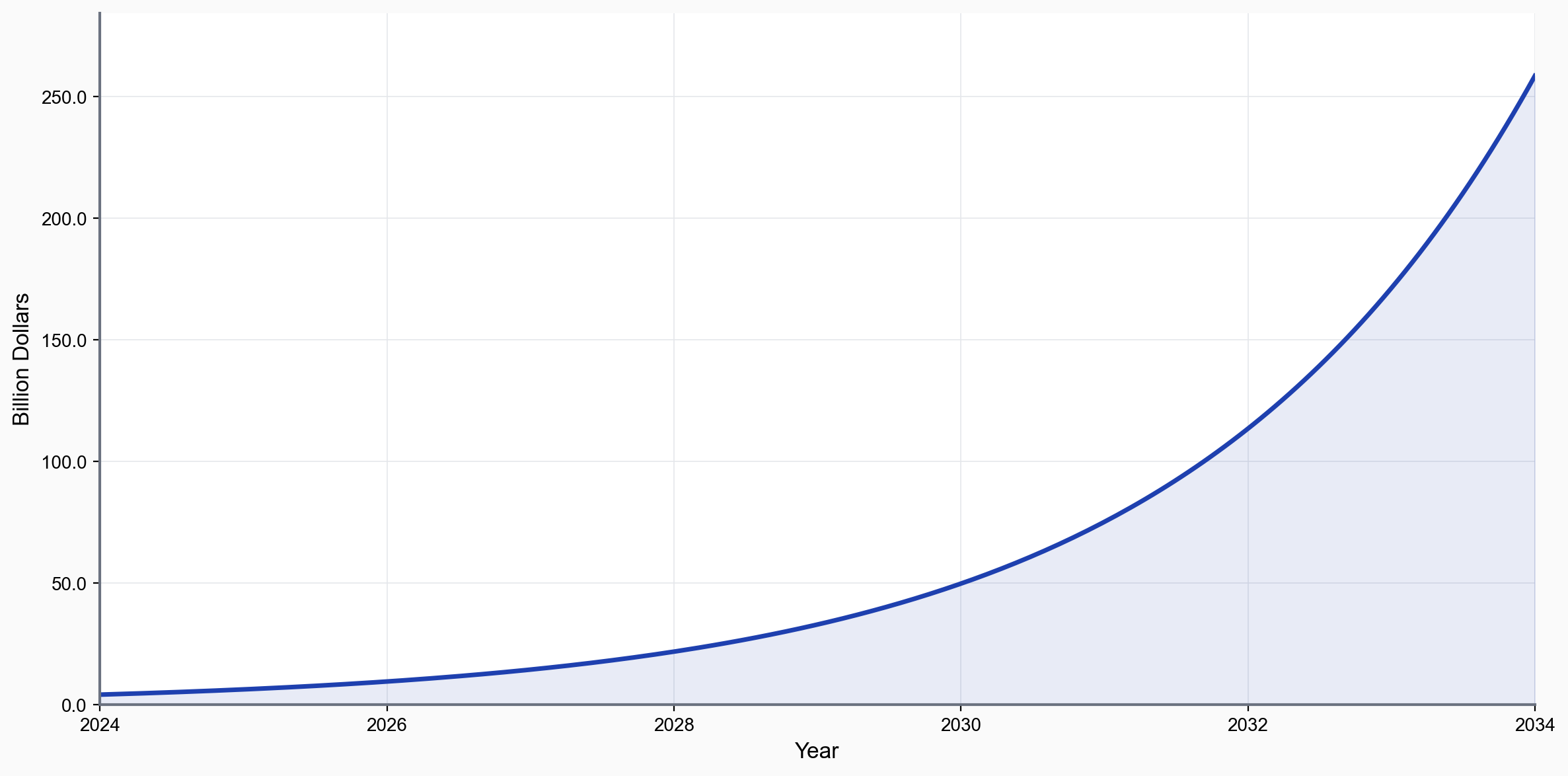
From a practical economic perspective, corporate investment in AI-related applications does not grow indefinitely but follows a logistical growth pattern driven by utility and risk assessment. As illustrated in Table 7, this trajectory is characterized by three distinct phases:
Initial Phase: Due to uncertainty surrounding the practicality and ROI of emerging AI tools, firms adopt a cautious approach with modest, exploratory investments, resulting in slow growth of .
Intermediate Phase: As the effectiveness of tools (e.g., GitHub Copilot, Gen-AI Agents) becomes evident, companies significantly increase capital allocation to capture competitive advantages, driving a rapid surge in .
Saturation Phase: Once AI tools have largely covered core application scenarios and investment reaches the enterprise's anticipated optimal scale, the growth rate slows and stabilizes, ultimately approaching a reasonable investment ceiling.
| Year | 2021 | 2022 | 2023 | 2024 | 2025 |
|---|---|---|---|---|---|
| Market Size (USD Billion) |
Note: Values for 2022 and 2024 are representative estimates derived from market ranges.
This slow-fast-slow S-shaped growth trajectory aligns closely with the intrinsic characteristics of the Logistic curve. We then construct a logistic function to map the original discrete observations into a continuous, smoothed temporal curve:
: The logistic smoothing diffusion rate coefficient for ,
: The inflection point of .
By applying the Non-linear Least Squares (NLS) estimation technique to the discrete dataset, we solved for the specific coefficients, yielding the following equation:
4.1.2 Logistic Regression
Similarly, follows a logistic growth trajectory comparable to the one discussed above. It begins with a slow initial phase due to low emphasis, accelerates rapidly as AI efficacy is proven, and stabilizes upon reaching an optimal saturation point. The corresponding modeling function is given by:
The meanings of and are similar to those of and .
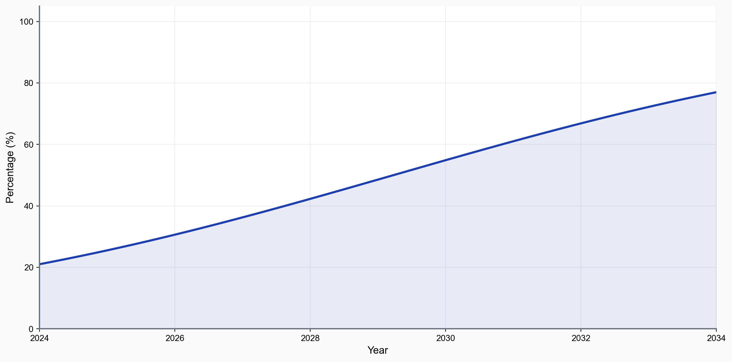
We utilized the NLS to perform parameter estimation on the observed data. The final regression model is derived as:
4.1.3 Linear Regression
In contrast to the logistic saturation seen in investment, AI skill demand exhibits a gradual rise. Given the extended cycle of workforce transformation, the market remains in an ascending phase without immediate saturation. Therefore, we approximate this trajectory as a linear model within our study's timeframe. The linear equation:
: the linear growth slope of .
: the linear intercept of .
We utilized the Ordinary Least Squares (OLS) algorithm to perform parameter estimation on the observed data. The resulting fitted function is given by:
4.1.4 Impact Model
After we have constructed models corresponding to the three indicators, we can now utilize these three indicators to forecast the Gen-AI impact rate. However, , and possess differing units of measurement. Therefore, we first standardize the function M(t).
We conduct a dynamic standardization method for AI investment amount , which calculates the current investment's progress towards achieving the target based on the projected ideal investment amount for 2034. By dynamically compressing the target time frame through the time adjustment factor , the target time is brought closer to the present. The resulting progress metric accurately reflects the investment progress as genuinely perceived at that moment and aligns with contemporary investment perceptions. is defined as:
: represents the investment growth curve we have estimated;
is a function that enables us to dynamically adjust the target time;
Based on the actual auxiliary effects of Gen-AI on professions and the characteristics of investment growth curves, we can assign flexible values to , dynamically narrowing the gap between the target time and the present. The resulting , expressed as a percentage between 0 and 1, standardizes the dimensionality while providing a realistic, normalized investment metric.
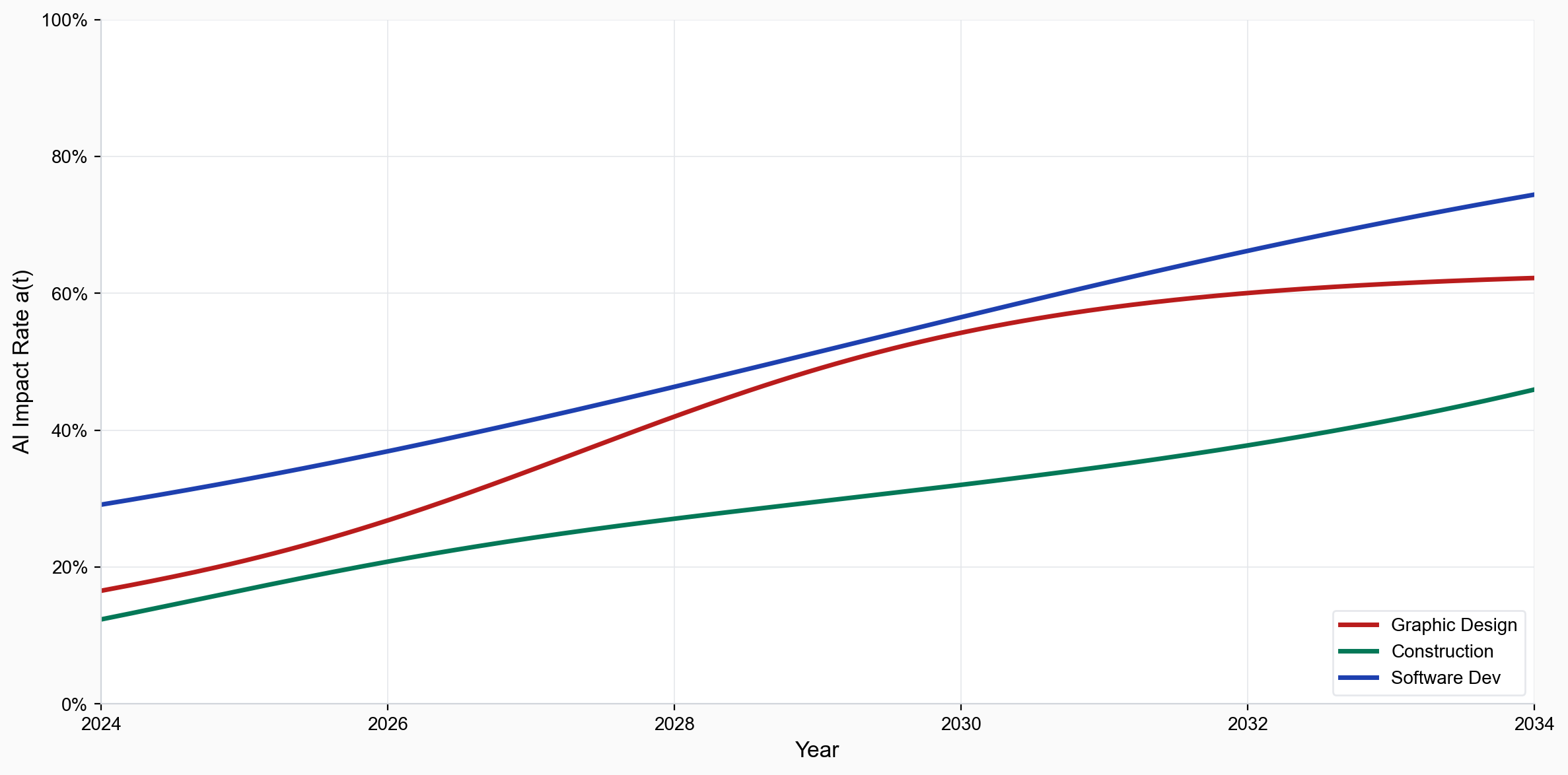
Subsequently, we can fuse the three standardized indicators according to their respective weights (calculated using the AHP) to obtain the final AI impact rate
4.2 Productivity Efficiency Model
Building upon the AI penetration rate derived from the previous step, this section establishes the Productivity Efficiency Model. This model translates the abstract penetration of technology into quantifiable gains in occupational productivity.
After forecasting the future impact rates of Gen-AI across three occupations, we task each profession with completing three identical types of professional tasks:
| Tasks | Sym. | Definition | Share | Efficiency Coef. | Time Reduction Factor |
|---|---|---|---|---|---|
| AI-Generable Tasks | Tasks that can be directly generated or fully automated by Gen-AI (e.g., coding, drafting). | ||||
| AI-Augmented Tasks | Tasks significantly enhanced by AI-assisted capabilities (e.g., data analysis). | ||||
| Human-Constrained Tasks | Tasks inherently bounded by human factors (e.g., negotiation, liability). |
To empirically determine task shares () and efficiency coefficients (), we established a computational pipeline that integrates granular occupational definitions from the O*NET Database with AI capability metrics from the Anthropic Economic Index.
Firstly, we mapped O*NET task descriptions to Anthropic's capability data using a three-stage cascade algorithm:
Exact Match: Direct string equality after normalization.
Fuzzy Match: Sequence similarity matching (Python
difflib) with a threshold of .Keyword Match: Jaccard similarity of semantic keywords with a threshold of .
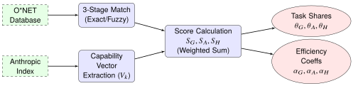
Secondly, we extracted the Anthropic capability vector for each matched task . We defined the raw scores for Generative (), Augmented (), and Human-Constrained () dimensions as:
Thirdly, we define that task shares for occupation are a weighted combination of the empirically matched data and a domain-specific fallback distribution:
Where is the normalized ratio of the summed scores across all matched tasks.
Fourthly, we calculate the efficiency coefficients. They are derived from the average intensity () of the relevant capabilities across the occupation. We construct bounded linear mappings to translate these intensities into time-reduction factors:
reflects high automation potential;
reflects moderate assistance;
reflects negligible AI impact on human-constrained tasks.
Finally, applying this pipeline to our three case study occupations yields the specific parameters listed in Table 8.
| Task Shares () | Efficiency Coeff. () | |||||
|---|---|---|---|---|---|---|
| Occupation | θ G | θ A | θ H | α G | α A | α H |
| Graphic Designers | 0.30 | 0.28 | 0.42 | 1.50 | 0.40 | 0.05 |
| Construction Mgrs | 0.13 | 0.30 | 0.58 | 0.80 | 0.40 | 0.03 |
| Software Devs | 0.22 | 0.51 | 0.27 | 1.20 | 0.50 | 0.05 |
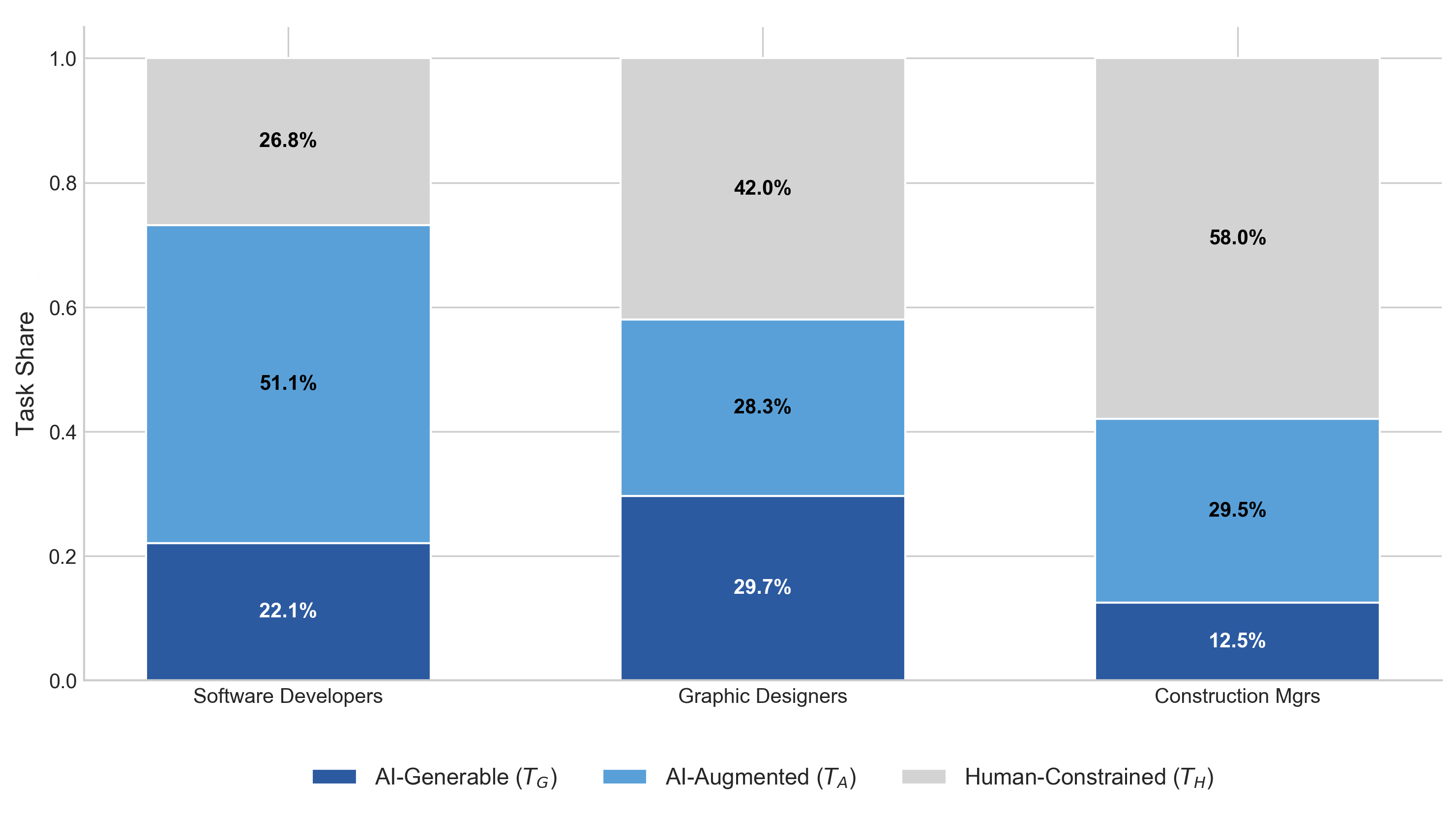
These parameters result in varying productivity trajectories. By 2034, Software Developers are projected to achieve a 33.7% productivity gain, whereas Construction Managers see a more modest 13.2% increase due to the bottleneck of human-constrained tasks ().
Once we have ascertained the values of the parameters, we derive the overall effective productivity improvement for profession :
Where reflects the proportion of effective working hours allocated to a particular category of tasks, representing the contribution of such tasks to the total working hours.
This model translates AI penetration levels into quantifiable gains in occupational productivity, precisely calculating productivity differences across professions at the micro-task level. It builds upon the AI impact rate and progresses to the output of productivity index . What's more, it calculates productivity based on task classification rather than entire occupations, reflecting the research logic that AI's impact on professions fundamentally stems from its influence on specific tasks within those occupations.
Taking Software Developers in 2034 as an example, with a penetration rate , the productivity index is calculated as:
This implies that a task package requiring 1 unit of time in 2023 can be completed in units of time in 2034, representing a 33.7% efficiency gain.
Similarly, we can calculate the productivity gains for the other two occupations, as shown in the table 9 below.
| Occupation | Penetration Rate | Productivity Index | Efficiency Gain |
|---|---|---|---|
| Graphic Designers | 62.2% | 1.270 | +27.0% |
| Construction Managers | 66.6% | 1.132 | +13.2% |
| Software Developers | 74.4% | 1.337 | +33.7% |
4.3 Job Vacancy Model
4.3.1 Baseline data
Firstly, based on employment data from the U.S. Bureau of Labor Statistics (BLS), we established a baseline employment trend . We applied linear interpolation to estimate the annual baseline employment in the absence of Gen-AI interference:
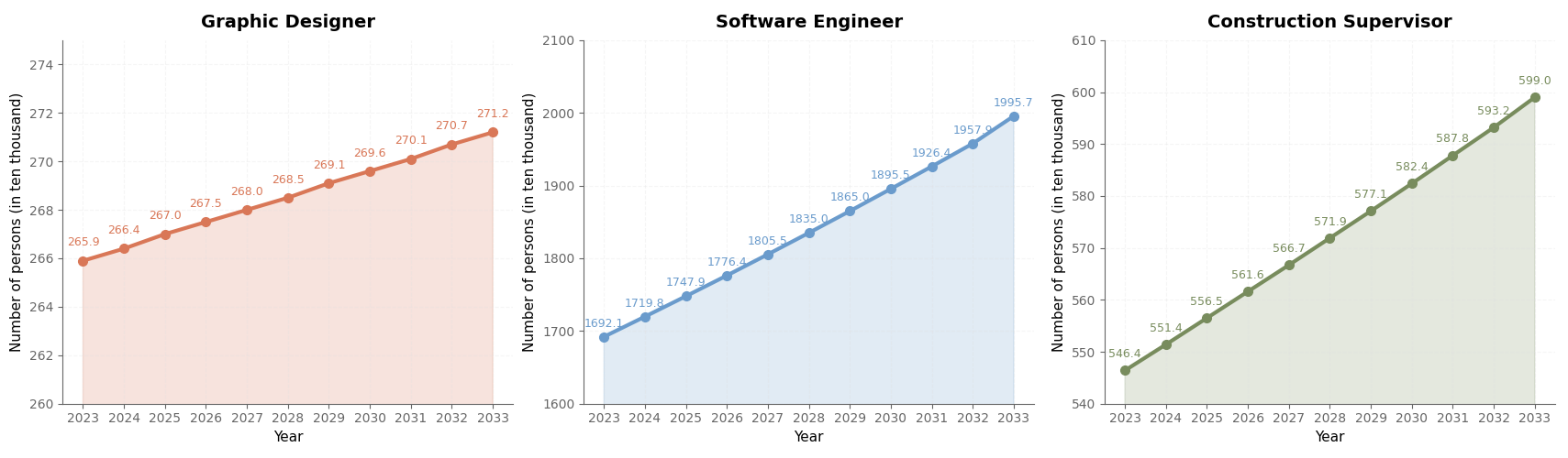
4.3.2 AI-impacted Employment
However, when productivity increases,like Gen-AI being applied to production activities, causing production costs decrease, and then employment demand may change. Therefore, we have established the following mathematical model to forecast changes in the number of jobs under the impact of Gen-AI:
Substitution Effect (described by ): As productivity rises, fewer workers are needed to accomplish the same workload. This force drives employment down.
Expansion Effect (described by ): Higher productivity reduces costs and improves service quality, which stimulates market demand. This force drives employment up.
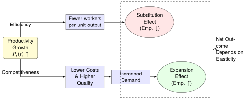
The parameter represents the Demand Elasticity of the occupation. It determines the net outcome of the supply-demand game. We calibrated based on industry characteristics:
High Elasticity (): Expansion Effect Substitution Effect → Employment increases
Low Elasticity (): Expansion effect Substitution effect → Employment decreases.
Moderate Elasticity: Expansion effect = Substitution effect → Employment remains unchanged
The values for different occupations are pivotal in explaining why, despite AI boosting productivity across the board, employment grows in some occupations while declining in others.
5 Courses and Admissions
5.1 Course Optimisation
This section proposes an institution-level curriculum redesign model that proactively reduces Gen-AI disruption to students and improves graduates' adaptability.
5.1.1 Decision Variables
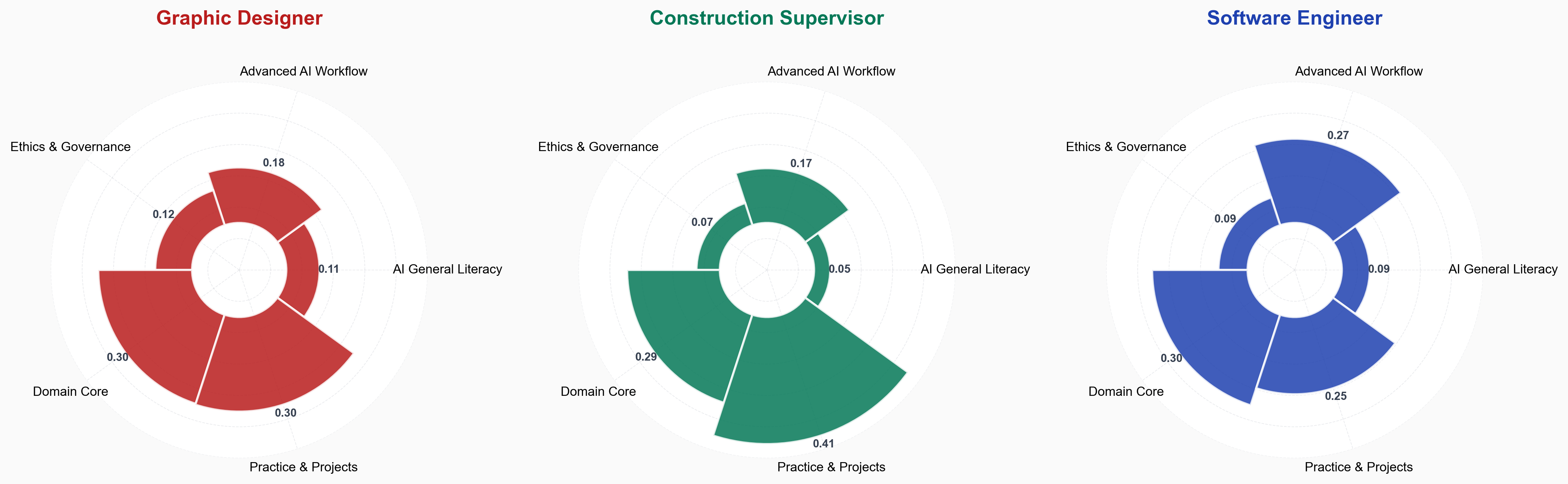
We allocate the total program contact hours into five components. Let be the share of total hours for occupation allocated to component ():
: AI General Literacy (Tools, productivity, information handling)
: Advanced AI Workflow (Profession-specific workflows)
: Ethics & Governance (Copyright, bias, compliance)
: Domain Core (Fundamental professional knowledge)
: Practice & Projects (Capstone, internship)
5.1.2 Optimization Results
We define an Adaptability Index to measure a graduate's robustness. It is a weighted geometric mean of learning saturation functions:
There are shared default learning-rate parameters:
Besides, we add a synergy term which ensures that AI skills () are only effective when backed by strong domain foundations ():
We then define the overall adaptability index using a weighted geometric mean:
The weights are generated from Chapter 4:
We set unnormalized weights:
Here is a governance-risk index (higher for occupations with stronger attribution risk);
allocates human-constrained requirements between domain core and practice.
We use shared constants:
and occupation-specific :
Using the selected occupations' task shares from Chapter 4:
The resulting normalized weights are:
For each occupation , we choose to maximize adaptability:
Software Engineer:
Construction Supervisor:
Graphic Designer:
We solve the smooth constrained optimization using the equivalent objective . The optimal curriculum hour shares are:
5.2 Enrollment Policy Adjustment
We translate the employment demand forecasts from Chapter 4 into actionable annual admissions targets.
5.2.1 Employment Demand Trajectories
Let denote the Employment Demand Model output for occupation in year .
Table 10 lists the provided values (2024–2034).
| Year | E GD ( t ) | E CS ( t ) | E SE ( t ) |
|---|---|---|---|
| 2024 | 261639.56 | 542788.57 | 1736468.17 |
| 2025 | 261278.12 | 545091.09 | 1768253.79 |
| 2026 | 260705.19 | 547570.17 | 1800522.46 |
| 2027 | 259992.59 | 550439.97 | 1833170.03 |
| 2028 | 259337.80 | 553654.82 | 1866057.84 |
| 2029 | 258912.06 | 557051.54 | 1899027.42 |
| 2030 | 258770.08 | 560469.69 | 1931919.40 |
| 2031 | 258871.08 | 563786.07 | 1964591.98 |
| 2032 | 259142.52 | 566907.90 | 1996934.79 |
| 2033 | 259520.55 | 569758.91 | 2028875.57 |
| 2034 | 259961.01 | 572269.17 | 2060379.80 |
5.2.2 Annual Entry Openings
Admissions should be aligned to the market's annual capacity to absorb new entrants. We therefore convert the stock level into annual entry opportunities via:
Where the first term captures employment growth (if positive), and the second term captures replacement openings due to separations (retirements, occupational transfers, etc.). We treat as a constant annual separations rate.
Default values used in computation:
5.2.3 Curriculum Reform as a Matching Gain
Section 5.1.2 produced an adaptability index for each occupation under its optimized curriculum. We convert this to a multiplicative matching advantage:
Where is a policy parameter representing the maximum achievable matching improvement from curriculum reform (default: ).
Using the Section 3.1 results:
We obtain:
We use two scenarios throughout:
S0 (Conservative): follow market openings only (no market-share gain), i.e., .
S1 (Reform Upper-Bound): curriculum reform yields the matching gain in Eq. (37).
5.2.4 Admissions Timing and Target Enrollment Index
Let denote the admissions year and let be program length for occupation :
Thus, admissions in year primarily affect graduation/entry in year .
We define an admissions index relative to the 2025 cohort:
We define the target index based on openings ratios. Let the baseline openings year be . Then:
5.2.5 Annual Adjustment Cap
To reflect capacity constraints, like faculty hiring lead time, capstone supervision and internship slots, we impose a hard cap on year-to-year admissions change:
We implement this with a clipping operator:
Where is either or depending on the scenario.
5.2.6 Admissions Paths
Applying Eqs. (35)–(45) to the provided series yields the following implementable admissions indices:
Software Engineer track:
Table 11. Admissions path for Software y t D ( 0 ) N ( 0 ) D ( 1 ) N ( 1 ) 2026 2030 1.0123 1.0123 1.1958 1.1000 2027 2031 1.0234 1.0234 1.2089 1.2089 2028 2032 1.0335 1.0335 1.2208 1.2208 2029 2033 1.0429 1.0429 1.2319 1.2319 2030 2034 1.0518 1.0518 1.2425 1.2425 Construction Supervisor track:
Table 12. Admissions path for Construction y t D ( 0 ) N ( 0 ) D ( 1 ) N ( 1 ) 2026 2028 1.0129 1.0129 1.1852 1.1000 2027 2029 1.0227 1.0227 1.1966 1.1966 2028 2030 1.0290 1.0290 1.2039 1.2039 2029 2031 1.0324 1.0324 1.2080 1.2080 2030 2032 1.0335 1.0335 1.2093 1.2093 Graphic Designer track:
Table 13. Admissions path for Graphic Design y t D ( 0 ) N ( 0 ) D ( 1 ) N ( 1 ) 2026 2030 0.9984 0.9984 1.1626 1.1000 2027 2031 1.0032 1.0032 1.1682 1.1682 2028 2032 1.0127 1.0127 1.1793 1.1793 2029 2033 1.0195 1.0195 1.1872 1.1872 2030 2034 1.0243 1.0243 1.1928 1.1928
6 Model Evaluation
6.1 Strengths
Data-Driven Design of Observable Proxy Metrics: The model employs three observable proxy metrics—AI-related investment amount , proportion of AI investment , and AI skill mention rate in recruitment advertisements —to construct AI penetration rate , thereby circumventing the challenge of difficulty in directly measuring true penetration rates. All proxy metrics are obtainable through public channels such as corporate investment reports and recruitment platform data, enhancing the model's reproducibility and practical applicability.
Methodological Adaptability and Innovation: Differentiated smoothing approaches are selected based on the growth characteristics of each proxy metric. S-shaped growth for and is modeled using logistic regression, while the progressive increase of 's incremental growth is modeled using linear regression, ensuring precise fitting of each metric's growth trajectory. The innovative introduction of a dynamic standardization method employing the time adjustment coefficient resolves the perspective misalignment issue inherent in traditional standardization, aligning the progress metric with real-time cognitive logic.
Adapting to Occupational Heterogeneity: Core parameters (time adjustment coefficient ) are occupation-specific, fully accommodating the differing AI impacts across STEM, trade, and arts occupations. For instance, trade occupations exhibit lower values, while STEM occupations demonstrate higher values. This alignment with real-world occupational characteristics enhances the model's interpretability.
6.2 Weakness
Proxy indicators exhibit limited coverage dimensions: The three categories of proxy indicators focus solely on corporate investment and recruitment demand, failing to encompass other AI penetration dimensions such as practitioners' actual frequency of AI tool usage or skill proficiency. Concurrently, proxy indicator data may contain biases, thereby impacting the computational accuracy of .
Parameter calibration exhibits subjective dependency: Although parameter fitting employs objective methods, the initial range for core parameters relies on industry reports or expert judgment. Different initial settings may induce model output bias, lacking a unified calibration standard.
External interference factors are insufficiently integrated: The model's core focus on the direct impact of Gen-AI overlooks external variables such as government AI policies, industry economic fluctuations, and breakthrough technological advancements. These factors may significantly alter AI penetration trajectories or employment demand, potentially introducing discrepancies between model predictions and reality.
References
U.S. Bureau of Labor Statistics. “Employment Projections: Occupational Projections and Characteristics (2024–2034).” https://www.bls.gov/emp/tables/occupational-projections-and-characteristics.htm ↗
U.S. Bureau of Labor Statistics. “Handbook of Methods: Employment Projections—Calculation (Occupational Openings / Separations).” https://www.bls.gov/opub/hom/emp/calculation.htm ↗
U.S. Bureau of Labor Statistics. “Occupational separations: a new method for projecting workforce needs.” Monthly Labor Review (2018). https://www.bls.gov/opub/mlr/2018/article/occupational-separations-a-new-method-for-projecting-workforce-needs.htm ↗
National Center for O*NET Development. “O*NET Database (Downloads and Documentation).” https://www.onetcenter.org/database.html ↗
Anthropic. “Anthropic Economic Index.” https://www.anthropic.com/economic-index ↗
Anthropic. “Which Economic Tasks are Performed with AI? Evidence from Millions of Claude Conversations.” (2024). https://assets.anthropic.com/m/7d3bfb95e798e00f/original/Anthropic-Economic-Index-Report.pdf ↗
Saaty, T. L. “Decision making with the analytic hierarchy process.” International Journal of Services Sciences, 1(1), 83–98 (2008). https://doi.org/10.1504/IJSSCI.2008.017590 ↗
Hwang, C.-L., and Yoon, K. Multiple Attribute Decision Making: Methods and Applications. Lecture Notes in Economics and Mathematical Systems, Vol. 186. Springer-Verlag (1981). https://doi.org/10.1007/978-3-642-48318-9 ↗
Acemoglu, D., and Restrepo, P. “Automation and New Tasks: How Technology Displaces and Reinstates Labor.” Journal of Economic Perspectives, 33(2), 3–30 (2019). https://www.aeaweb.org/articles?id=10.1257/jep.33.2.3 ↗
National Center for Education Statistics (NCES). “Glossary: Degree-granting institutions.” https://nces.ed.gov/ipeds/glossary/?charindex=D ↗